
Natural language processing revisited
5 February 2015
There is a very interesting course on Natural language processing on youtube, it is by Prof. Dan Jurafsky & Chris Manning.
i took some notes while watching these lectures (they are here at the end of this article);
Now some twenty years ago i attended a course on natural language processing and so to me it was very interesting to see how the field has progressed.
Things that changed are
- renewed interest in dependency grammars
- strong focus on commercial applications, previously the focus was on demonstration systems; demonstration systems are build with the limited purpose of demonstrating the feasibility of a concept, so they are much less robust than commercial applications ;
- nowadays there is a strong interest in models that are based on probability
- corpus based approach to evaluation of result
Natural language processing is a very interesting field of study as it combines some linguistics, statistics/information theory/machine learning, programming and AI tricks.
interest in dependency grammars
For a very long time, up until the late nineties, there was this strong focus on Context free constituency grammars - these are similar to BNF rules that define the syntax of a programming languages: in both cases the inner node of a parse tree is just the name of a abstract category - for a given sentence, the type of inner node is determined by the production rule that can be applied to parse the sentence; the inner nodes of the parse three knows nothing about the leafs of the tree.
The problem with this approach is that it produces very deep tree structures and it is very hard for a program to assign a meaning to such a complex structure; Another point is that the grammar grows quite complex as it has to be able to describe all possible cases of correct utterances, a complex grammar makes an even more complex parse tree; also this complexity of grammar turns parsing into a challenging and time consuming task; Still another problem: it is very hard to formulate a grammar for languages with relatively free word order.
Nowadays there is a renewed focus on dependency grammars; (see lectures here and here and here ) Here instead of abstract categories without context there are head words (with the main verb ending up as the highest level node)
The result is a more shallow parse tree; for a program this makes it much is easier to interpret such a structure: a head verb can be mapped to a function that does an action, all subordinate clauses are then just argument to the procedure that stands for this action.
(incidentally context free grammars evolved into this direction: in modern context free grammars the categories are annotated with the head word: (see x-bar theory and lexicalized context free grammars), however the parse tree here remains more complex, even in its modern form
Now this is not quite new; the SHRDLU program written in 1972 by Terry Winograd did have a similar structure: (here is Winograd’s dissertation that describes this program)
The user of the program enters phrases in English that talk about geometric objects on a table: like here
Like this one
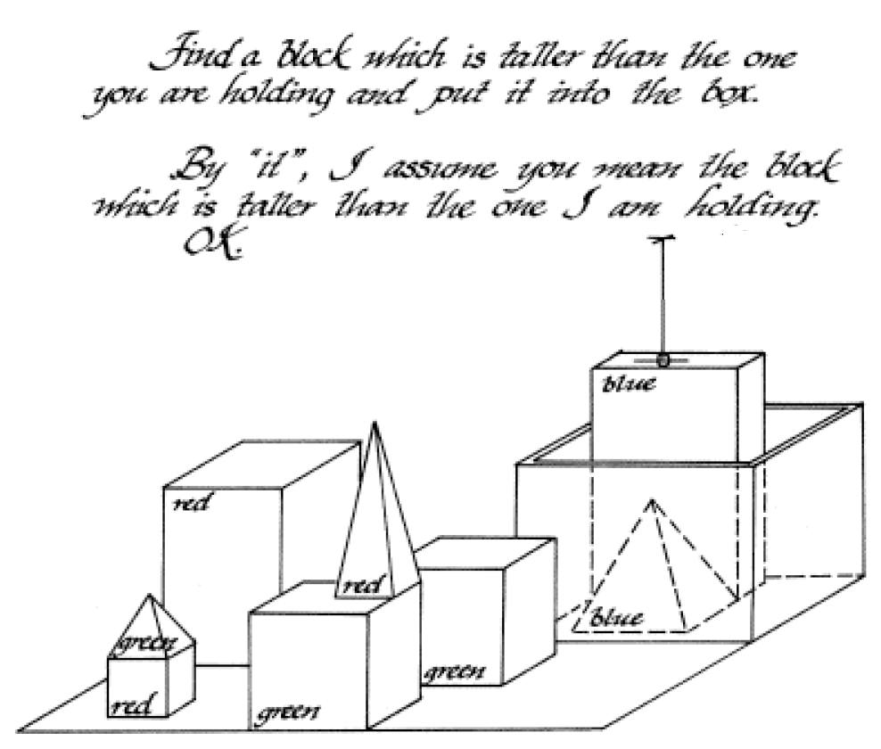
The program creates a database entry for each geometric object that is mentioned, this database bentry lists properties of each object, like color, shape, position of the object relative to other objects on the table. It can change the properties of its database entries according to the requests that are typed in in English; it also answers question in English . It is also drawing a picture that contains all of the objects that it knows about. In the picture thereis also an arrow that points towards the block that the program is ‘holding’)
The input sentence is parsed according to a systemic grammar; this grammar also produces a relatively shallow parse tree where the verbs are directly mapped to procedures that handle the input text;
However this program was ignored by the linguists of MIT; practical considerations that were required to build computer systems, like depth of the parse tree, were of not interests to them.
strong focus on commercial applications less focus on preset notions
Once upon a time artificial intelligence research was funded exclusively by the US military, by means of programs like ARPA/DARPA. The ‘golden days’ of artificial intelligence were in the sixties to mid-seventies, when US research spending was were very high in general because of the space race.
Research was centered around a few university departments at top universities like MIT, Stanford etc; Each research department was led by a strong personality who would organize the funding and who could formulate a general approach to his area of studies (like the “Syntactic Structures” of Noam Chomsky)
Terry Winograd in this interview here
TW: And of course at MIT, there was a huge amount of syntax, but that was another one of these sort of feuding worlds; you couldn't talk to Chomsky and Minsky both, it was impossible. The one contact I had is I went and took a course from Chomsky, wrote a term paper saying why I thought this AI-ish approach would work, and he gave me a 'C' on the term paper. That was the end of my contact with the Linguistics Department.
Also here
TW: Minsky and Chomsky were both very strong personalities. You could go to one or the other but you couldn't be in the middle. That is how MIT is, it has strong boundaries between its departments. MV: But you were allowed to do computers and linguistics? TW: Minsky wanted me to do linguistics and prove that his students could do better linguistics than Chomsky's. I was not the first. Dave Waltz, who eventually went on to do work in vision, was doing a research project on linguistics when I got there, as was Gene Charniak. And in the prior generation Daniel Bobrow and Bertram Raphael had both done language projects. So it was a major stream of work in the AI Lab."
One would have expected that this setting would lead to personal fiefdoms, one of the features of such an organization is that everyone is protecting his own turf and not eager to cooperate. Now what they had at MIT’s AI lab was just the opposite; Researchers had a lot of autonomy with regards to their projects; the people who were in esteem where the programmers/Lisp hackers; also they developed a culture of information sharing and cross boundary cooperation.
"WINOGRAD: It was people who were basically working on their own and then knowing enough about what each other was doing to join up. So, for example, this stuff on Micro-Planner was useful for all three of the people who did it, so we got together and did that. And to comment, and so on. I probably saw Marvin - well, he wasn't actually my official advisor, Seymour was, but I don't think I saw either of them to talk about my dissertation more than once every few months. It wasn't like they were directing the project."
another point is that the research departments were producing demonstration systems of simplified domains (like the block world in SHRDLU), not actual products:
Implementation meant something you could show off. It didn't mean something that somebody else could use. So - I mean, my thesis was certainly that way. I mean, you know, the famous dialogue with SHRDLU where you could pick up a block, and so on, I very carefully worked through, line by line. If you sat down in front of it, and asked it a question that wasn't in the dialogue, there was some probability it would answer it. I mean, if it was reasonably close to one of the questions that was there in form and in content, it would probably get it. But there was no attempt to get it to the point where you could actually hand it to somebody and they could use it to move blocks around. And there was no pressure for that whatsoever. Pressure was for something you could demo. Take a recent example, Negroponte's Media Lab, where instead of "perish or publish" it's "demo or die." I think that's a problem. I think AI suffered from that a lot, because it led to "Potemkin villages", things which - for the things they actually did in the demo looked good, but when you looked behind that there wasn't enough structure to make it really work more generally.
This changed: the personal computer and wide spread adoption of the Internet created many commercial applications of natural language processing; the result was that a lot of focus shifted towards the research divisions of Microsoft, IBM and Bells Labs.
These applications were:
-
spelling checkers for word processors
-
spam detection for email systems
-
information retrieval systems for WEB search.
- speech recognition
- question answering / text classification /sentiment analysis / relationship extraction / etc. etc.
I guess that these new requirements generated a shift in priorities: now the dominant explanation would be the one that could be used to build a working system, not the ones who would correspond to preset notions of how things were to be explained.
Also the natural language processing course that i did some twenty years ago was not very well attended, however i guess that this would have been different if students could have been able to predict that this field would create the biggest software company in the word.
New focus on probabilistic models
Since the fifties probabilistic models were used in information retrieval, however in the study of grammar they were not very much used.
I guess this was due to opposition by Noam Chomsky;
Peter Norvig and Prof. Noam Chomsky are debating this issue here
Chomsky’s argument is quoted as follows: “It’s true there’s been a lot of work on trying to apply statistical models to various linguistic problems. I think there have been some successes, but a lot of failures. There is a notion of success … which I think is novel in the history of science. It interprets success as approximating unanalyzed data.”
Chomsky argues that statistical models do not add insight; Peter Norvig cites many examples where statistical meaning did add insight in physics and of course sites many successful systems that utilize this technique.
The debate does not mentioned the following: Chomsky established his approach as an opposition to previous behaviorist explanations of language acquisition; Skinner argues that children learn language by associating words with meaning; here good performance is encouraged by correct behavior (reinforcement principle); Chomsky argues that this stimulus cannot explain how a child manages to acquire language in such a short time; he argues that humans come with a built in facility of understanding language called universal grammar, so language acquisition is just a process of applying these general principles;
Now Chomsky is trying to identify and understand these Universal principles by means of introspective reasoning; Interesting, another possibility would have have been a more empirical approach: use statistics in order to study language acquisition patterns and use that in order to discern universal principles; Now the problem is that this is that statics are the favorite method of behaviorist psychologies, and Chomsky established his paradigm as opposition to this approach.
However nowadays it is more important to produce working systems, and theoretical considerations of this kind seem to be less important than that.
corpus based approach to evaluation of result
Now every algorithm is tuned over a hand classified text set (corpus). For parsers there is always a tree bank - a set of sentences that has been parsed into either a constituency tree or dependency graph. Part of this data is used as the training set - the set of data to tune the performance of an algorithm; the other part of this data is used for evaluation of performance.
One practical problem is that this data costs a lot of money - so they do maintain some artificial barriers of entry; however some of the data for some languages is available with an open source license (see here )
Another problem is that the selection of the test data may also constitute some form of bias on its own; for example parser treebanks are not that large because the task of hand parsing of the text is a bit complex; POS pre-tagged corpus is larger; as the task of hand tagging is easier.
Lecture notes on Natural language processing course by Prof. Dan Jurafsky & Chris Manning.
(2 - 1 - Regular Expressions)
- uses regular expressions to parse tokens; uses http://regexpal.com to show regex syntax (Yawn).
-
edits regular expression to fix problems:
- Increase accuracy/precision to exclude strings should that not have matched (False positive Type I)
- Increase precision to include string we should have matched (False negatives - Type II)
- regular expression matching is often the first model of any text processing task; or as first stages for more complex processing.
(2 - 2 - Regular Expressions in Practical NLP)
- English tokenizer in Stanford NLP library; written in jflex lexer. (java version of unix tool flex)
covers lots of conventions: like:
(acronyms as regexes) ABMONTH=Jan|Feb|March …
show regex for phone numbers (quite complicated - parse country extension, etc. lots of special cases, like regex for parsing email addresses)
(2 - 3 - Word Tokenization)
-
Lemma: share same stem + part of speech (cat , cats)
-
word form: inflected ‘surface form’ - cat,cats are different word forms.
-
counting words: are fillers/fragments like Ah,Uh counted as words? counting tokens? or number of dictionary entries? or number of lemma’s
-
convention N - number of tokens V number of dictionary entries (vocabulary size) -
how big is vocabulary of a corpus? Church&Gale estimate V > O (SQRT( N )
examples of fiddling with unix command pipelines:
| tr ~~sc ‘a-zA-Z’’\n’ | sort | uniq # turn non letter characters to newlines (what about i’m~~> i + m) then sort then remove repetitions. |
| tr -sc ‘a-zA-Z’’\n’ | sort | uniq | sort -n -r # now sorts by frequency |
| tr ‘A-Z’ ‘a-z’ | tr -sc ‘a-zA-Z’’\n’ | sort | uniq | sort -n -r # now does it case insensitive (turn to lower caps) |
other problems:
-
now Finland’s -> Findland + s ; state-of-the-art -> state + of + the + art; m.p. -> m + p
-
compound word segmentation (German); French: L’ensemble
-
segmentation of tokens in Chinese+Japanese (no spaces)
-
(use matching of longest dictionary entry at cursor
- this wouldn’t work for English without spaces - more ambiguous choices)).
- Japanese + mix of different alphabets.
(2 - 4 - Word Normalization and Stemming)
-
‘normalize’ after tokenization - this means different things
- for information retrieval: input query token must match the internalized representation of data in a program (example: delete punctuation from input query , to lower case (search engine indexes words in lower case form only), etc.)
-
however case may be needed to distinguish between acronym and real word (for example)
- lematization: remove inflection (am,are,is
be ; car cars> car)
for reduction to lemma we need Morphology:= smallest unit that make up words (stem, affixes) stemming := removal of affixes
Porter algorithm for stemming of English words
Step 1: catscat (suffix, lots of rules) Step2) walking>walk (lots of rules like only apply if vowel before -ing); etc. etc. (well it gets rather hairy, with lots and lots of rules)
(2 - 5 - Sentence Segmentation)
How to divide text into sentences: good markers for end of sentence are ! ? however . - is ambiguous.
Need to decide if . is end of sentence - classifier: decision tree.
    lots of blank lines after?

        /   \
       no-eof-s final punctuation is ? or !
                \
                final punctuation period?
                /                     \
            is final word an abbrev.     is-eof-s
            /   \
            no-eof-s    ???
-
can use probability: is this word likely to appear at end of sentence? or this this likely to be an abbreviation?
- problem: simple decision trees with few rules are hand coded;
- complicated trees with numeric thresholds for probability - that’s where machine learning comes in.
(3 - 1 - Defining Minimum Edit Distance)
-
measure similarity of strings = minimum number or edit operations (character insertion,deletion,substitution) to transform string A into string B
-
Levenstein distance: insertions + deletions cost 1; substitutions cost 2.
string [a1……an] and string [b1….bn] (two sequences of characters)
D[i,j] = cost of transformaing string [a1….ai] into string [b1….bj]
if a1…ai and b1….bj are equal except for one character than
Recurrency - compute edit distance from edit distance of shorter strings.
    D[i,j] = MAX(  D[i-1,j] + 1 # inserting character to a (a becomes longer to match b)
               D[i,j-1] + 1 # deleting character from a (becomes shorter)
               D[i-1,j-1] + 2  (if a[i] != a[j] # substitution costs 2
               D[i-1,j-1] + 0  (if a[i] == a[j])    # nothing to do.
             )
D[I,0] = i # must delete all characters to transform a1…aj to null string
D[0,j] = j # must insert all characters to transform null string to a1…aj
Now table can be filled, with complexity O (i * j)
(3 - 3 - Backtrace for Computing Alignments)
alignment: did the character in target string come from the source string? for each D[i,j] remember previous actions that lead to it + applied change. (if it came from D[j-1,j-1] - because last char was a fit or not)
(3 - 4 - Weighted Minimum Edit Distance)
-
assign different weights to different substitutions. Why?
-
some spelling errors are more likely than others (like confusing vowels); in biology some transofmrations of DNA are more likely than others
    D[i,j] = MAX(  D[i-1,j] + InsertionCost( xi )   # function returns cost of insertion for character xi
    `          D[i,j-1] + DeletionCost( yj )    # function returns cost of deletion for character xi
               D[i-1,j-1] + SubstitionCost( xi, yj ) # function returns cost of substituting character xi with xj
               D[i-1,j-1] + 0  (if a[i] == a[j])    # nothing to do.
             )

    D[I,0]  = D[i-1,0] + DeletionCost(xi)


    D[0,j]  = D[0,j-1] + InsertionCost(yj)
Richard Bellman: says that name ‘Dynamic programming’ came as a marketing trick, as then secretary of defense did not like math research.
m(3-5-Minimum Edit Distance in Computational Biology)
- compare geneses from different species - to find important regions/identify functions/see how things changed.
Terminology in biology: editing distance <> sequence similarity; weights <> scores
- in biology its OK to have unlimited gaps at start and end of a sequence.
(4 - 1 - Introduction to N-grams)
Language model - assign probability to a sentence (one application: score sentences that come out of machine translation (???); spelling correction, speech recognition - find the more likely interpretation).
p(W) = P (w1 … wn) - the probability of sequence of words. P (W5|w1…w4) - probability that w5 follows w1…w4. (aka. probability of upcoming word)
Language model - computes both probability of sequence of words + probability of upcoming word
| P (A | b)= P (A n B) / P (B) ; |
| (i always understood it in terms of the classical definition of probability P (A) = | A | / | all | ; here this means P (A | B) = | A n B | / | B | as | all | is canceled out; ( set picture + probability of a given b = frequency of both a and b divided by frequency of B); don’t know why this works for all probability measures) |
| P (A n B) = P (A | B) P (B) |
chaining rule:
| P (An n … A1) = P (An | An-1 n …. A1) P (An-1 n …. A1) | ||
| P (An n … A1) = P (An | An-1 n …. A1) P (An-1 | An-2…A1) P (An-3 | An-4 n …. A1) …P (A1) |
| How to compute P (An | An-1 n …. A1) for a long sentence? |
| Markov property: P (An | An-1 n …. A1) ~ P (An | An-1 n …. An-m) (a shorter sentence will be a good approximation) |
Markov property says that a process is ‘memory less’ - it depends on the preceding state, but can do with the recent state, as long past events have diminishing effect/impact.
Unigram model = just look at previous word (assume Markov property of m=1) : P (A1 n … An) = P (A1) … P (An) ;
If this model is used to create random sentences: not very good it assumes that words appear independently of each other.
| Bigram model: P (A1 n …. An) = Product of P (An | An-1) over n |
If this model is used to create random sentences: does much better than unigram modell.
Still n-gram models are insufficient because of long distance dependencies between subject and object; for some application local context is good enough.
(4 - 2 - Estimating N-gram Probabilities)
- count frequency of each bi-grams (two word sentence) in huge corpus (text collection) in order to get probability of bi-brams. (also need count of single words - unigrams)
P (W1 n W2) = countOf(W1 W2) / count(W2)
- column and rows are words of matrix; it holds count of occurrences for each bigram. sparse matrix (lots of possible bi-grams never occur)
    P(I want money) = P( I) P(I want) P(want money) P(money )  | I - I at the start
    of a sentence ; money  # money at the end of a sentence.
-
some bigrams occur/do not occur because of grammar (allows/disallows); some because of peculiarities of the studied corpus (text set).
-
everything added as logarithm ( p1 * p2 .. pn = log(p1) + log(p2) … + log(pn) (avoids underflow and is faster)
-
toolkits for this: SLIRM ; google n-grams (even has four-grams); google book n-gram (corpus from google books)
(4 - 3 - Evaluation and Perplexity)
-
measure the accuracy against text data that is not in the training corpus (the text that was used to compute the n-gram probabilities)
-
model can be used in task (such as spelling correction) then see how many errors. (aka extrinsic (in-vivo) evaluation)
intrinsic evaluation
perplexity - how well can we predict the next word? (aka shannon game)
- perplexity PP (W) = ( p(w1,w2,….. wn) ) ^ (1/n) (normalized (^(1/n)) of words)
The lower the perplexity - the better the model.
-
as the model for n-grams is a product, then perplexity is just the mean probability of each bi-gram
-
another description of perlexity: branching factor; at each word position, how many choices are there?
(4 - 4 - Generalization and Zeros)
-
Shannon visualization method: generate random sentences from the n-gram model.
-
if you take Shakespeare corpus and wall street journal corpus for this generation: no overlap in generated sentences.
-
(for Shakespeare corpus 99.6 of all possible bi-grams did not occur) -> n-gram model only works good for text that is similar to the training corpus.
-
problem if bi-gram did not occur in test set then probability of it is 0.
-
want to assign some probability to non occurred bi-grams: La-place smoothing - add one to all occurrence counts.
| P (wi | wi-1) = (count(wi wi-1) + 1) / (count(wi-1) + V) (V - vocabulary size) |
-
now if we get the counts for changed probabilities - it changes them significantly; add one smoothing is not used for n-grams.
-
-> smoothing is ok for text categorization, but not for modeling.
(4 - 6 - Interpolation)
-
backoff: example there was a tri-gram with count 1 (so no much confidence in the data) -> so use bi-gram instead.
- interpolation: mix unigram, bi-gram and tri-gram - so composite of the data is used all the time.
- Linear interpolation
| P (wn | wn-1 wn-2) = Lambda1 P (wn | wn-1 wn-2) + Lambda2 P (wn | wn-1)+ Lambda3 P (wn) |
add weight1 * tri-gram probability + weight2 * bi-gram probability + weight3 * unigram probability; sum of weights has to be 1 (to remain a probability measure)
-
weights conditional on context: weight is not constant, it is a function on the previous word (can be ‘trained’ better)
- now there is
- training data: - corpus for getting n-grams
- held-out data - corpus used to tune the weights
- test data - used for check
-
search for weights that maximise the log probabilities for held-out data set (?)
- what if word is not in corpus? have sepcialtoken
to mach all unknown words - from corpus take out a fiew rare words and reassign their probability to Unk; then get the n-grams probabilities (train the n-grams)
-very large corpus (like google n-gram) what to do?
-
one possibility is pruning (only store n-grams with count > threshold)
-
or omit based on entropy measures (more sophisticated then count only)
- other tricks: use ‘smart’ data structures (tries); do not store strings, store index numbers of strings; use huffman coding;
- Backoff (use of bi-gram instead of three-gram) for web scale: Stupid backoff (does not produce probabilites !) W (n)(i-k+1) - sequence of n words starting ending at position i in the text
// if both current ngram and shorter ngram (shorter by one word) appear -> take the ngram if (count(W (n)(i-k+1)) / count( W (n-1)(i-k+1) ) then return count( W (n)(i-k+1) ) // else take count of the shorter n-gram with factor 0.4 else return 0.4 * count( W (n-1)(i-k+1) )
Count( W (i)(i-k+1) ) / count( w(i-1)(i-k+1) > 9
- recent research: discriminative models: choose n-gram modell to improve a given task (not based on corpus?)
- caching modell: a recently used word is likely to appear again; so use probability measure that factors in recent usage. (doesn’t work good for speech recognition)
(4 - 7 - Good Turing smoothing)
what is the probability of an unseen/unknown word?
-
count N1 = | n-grams that occurred once | (class c = 1) N2 = | n-grams that occurred twice | (class c = 2) …..
- probability that next word is unknown is equal to probability of n-gram that occured once;
-
but we need to adjust the probabilities of the remaining classes ! (otherwise it does not sum up to one - and it is no longer a probability measure).
-
modified count NewNC: NewNc = ((c+1) N (c+1)) / Nc
- ? did not quite understand how this works out ?
(4 - 8 Kneser-Ney smoothing)
-
in practice Good Turing is supposed to change most occurance counts by some fixed amount (- 0.75 ? )
-
so apply the idea of a ‘discount’
| P-abs-discount( wi | wi-1 ) = ( count( wi-1 wi ) - d ) / count(wi-1) ) + Lambda(wi-1) * P (W) |
P (w) - (unigram probability) Lambda(wi-1) - weight function takes previous word as input.
-
problem: unigram probability is without context, so does not say much; high probability word that can appear out of contest is best fit.
-
Kneser-Ney smoothing: something better instead of unigram prob.
-
should be proportional to number of different n-grams that end with a given word w = { wi-1 : c(wi-1,w) > 0 } -
number of all different bigram types - { wi-1,wi : c(wi-1,wi) > 0 }
| use P-continuation(w) := | { wi-1 : c(wi-1,w) > 0 } | / | { wi-1,wi : c(wi-1,wi) > 0 } |
- Kneser-Ney looks like:
| P-abs-discount( wi | wi-1 ) = Max( count( wi-1 wi ) - d, 0 ) / count(wi-1) ) + Lambda(wi-1) * P-continuation(W) |
Lambda(wi-1) - uses constant d to cancel out d discount and reassign probability to P-continuation factor.
| Lambda(wi-1) := (d / count(wi-1)) * count( { w : count(wi-1,w) > 0 | ) |
(d / count(wi-1)) - second term when you open up the fracture expression count( { w : count(wi-1,w) > 0 |) - number of bi-grams that start with wi-1 == how many times was d discount applied
- full recursive form (for all n-gram types) is very involved …. (TBD)
(5 - 1 The spelling correction task)
- types of errors: non word errors real word errors
- typographical errors (misplaced a letter and real word turns up)
-
homophones - cognitive errors)
-
fixing non word errors: find candidate fixes by dictionary lookup, pick up the words with shortest edit distance or highest noisy channel probability (see further down)
- fixing real word errors:
candidate set = find words with similar pronunciation and spelling and also include the input word in this set.
pick suggestion - noisy channel model/classifier.
(5 - 2 Noisy channel model)
-
noisy channel - input runs through a distorting communication channel; builds a modell of the distortions from the output errors.
-
decoder: runs input words through the noisy channel model - if output distortion is nearest to given observed signal (from the output end of the channel) then given input word is the match.
-
Noisy channel: given misspelled word x find correct word w
| argmax P( w | v ) # find word w that maximizes probability of word given misspelling (max over all words of vocabulary) |
| argmax (P( x | w ) P (w)) / P (x) = # use bayes to express in terms of misspelling given correct word |
| armax P (x | w) P (w) # P (x) is constant so it (does not contribute to maximum ?), cancelled out |
P (x|w) - likelyhood P (w) - prior
| P (x | w) P (w) = language model/channel model/error model |
correction candidate generation: need either small edit distance or small distance in pronunciation.
Demerau Levenstein edit distance
for spell correction also has transpositions of two letters (in addition to insertion/deletion and substitution)
-
big assumption: 80% of errors within edit distance 1 (or two) (? what about dyslexia, also why is it assumed that everybody does the same errors ?)
-
should also allow for insertion of space/hypen.
= Channel model details: what are likelyhood of partial edits? del[x,y] = countof( xy typed as x) ins(x,y) = countof( x typed as xy) sub(x,y) = countof( x typed as y ) trans(x,y)= countof( xy typed as yx)
(empirically compiled these, as usual)
P (x|w) - if deletion: del(wi-1,w) / count(wi-1,w) if insertion: ins(wi-1,xi) / count(wi-1) if substitution: sub(xi,wi) / count(wi) if transposition: trans(wi,wi+1) / count(wi,wi+1)
-
unigram model for prior (P (w) factor in language model) can make mistakes; use ngram instead (do P (wi+1 w) and P (w wi-1)
(5 - 3 Real - Word spelling)
-
real word errors (mixing up two words that are correct, homophones or misuse); tougher to solve (about 40% of all mistakes)
-
for each world generate candidates: the word itself, homophones; words that have short edit distance to input word.
-
the right sentence could be any path (each one chosen from one candidate set); choose the most likely choice; Assumption: (again) there is one misspelled word in sentence (???)
-
use same channel modell (likelyhood of error edit) + n-gram language modell to check likelyhood of result; need probability of no error (assumption by application) (90% correct ???)
(5 - 4 State of the art issues)
-
problems addressed in real systems:
-
(UI issues) auto correction if have high confidence; user choice on less confidence; flag as errors if very low confidence.
-
channel model in practice: lots of seperate/not quote correct assumptions happen when likelyhood (P (x w)) is multiplied by Prior (P (w)) (all lies); so weight them. argmax P (x w) * (P (w) ^ Lambda) # Lambda is tuned (trial error).f -
pronunciation similarity is also often used (not just edit distance). (Aspell uses GNU Metaphone to transcribe words) ; have to combine these factors.
-
allow more edit primitives: ph -> f ; ent -> ant
-
other factors might be considered in channel model: position in word; surrounding letters; nearby keys on keyboard; morpheme transformations (like ph -> f ; ent -> ant)
- combination of factors done by classifies (more explanation in next video)
(6 - 1 Text classification)
-
Tasks:
-
task of deciding if email is spam; (identify fishy attributes ! in title, fishy url …)
-
task of authorship attribution (deciding who was the author based on writing style - Bayesian methods)
-
gender identification (Female authors tend to use more pronous; male more determiners,facts (??))
- sentiment analysis: tell if a review is positive or negative?
-
scientific articles: what are the key-words of an article? subject categories?
-
given text document d ; and categories C1…CN; assign category Ci to d.
-
can be done by hand written rules (if,then,else (many recursions)) problem: expensive.
- general approach: supervised machine learning: Input: set of classes c1…cn set of training documents d1…dm; Ready assignment of documents (trainingset) di->dj Output: a classifiert that assigns di to class cj
(6 - 2 Naive Bayes classifier)
- Bayes classifiers: approach is to look at the text as bag of words: only extract words deemed significant and omit all the rest; order of words does not matter (count of repetition does apparently)
(6 - 3 Formalizing Bay es)
| P( c | d ) = (P (d | c) * P (c) ) / P (d) |
| P( c | d ) - prob. of assigning given document to given class. |
Now can do the usual
| find: for all classes c: maximumfor-all-c P (c | d) = max-for-all-c (P (d | c) * P (c) ) / P (d) = |
P (d) is constant, so that maximum without this division is also the real maximum
| = max-for-all-c (P (d | c) * P (c) ) |
–
P (c) := the likelyhood that a document d belongs to class C.
| P (d | c) := by bag of word analysis we only look at set of words x1…x2 from d; |
| P (d | c) = P (x1….xn | c) |
also assume that probabilities for x1..xn are independent (not correlated) (another oversimplificiation)
| P (x1….xn | c) = P (x1 | c) * .. * P (xn | c) |
So: P( c | d ) = max-for-all-c P (x1|c) * .. * P (xn|c) * P (c)
(6 - 4 Naive Bayes learning)
P (cj) = countof(Cj) / Ndoc # divide number of docs of class j by number of all docs.
| p(wi | cj) = count(wi, cj) / Sumof-over-c count(wi, c) # divide (count of word wi in documents of one class cj) by (count of word wi in all document classes) |
-
Problem: can’t use it that way; if count(wi,cj) 0 then probability P(wi cj) 0; then the whole product of word probabilities turns 0; (useless). - solution: use smoothing
| p(wi | cj) = (count(wi, cj) + 1) / (Sumof-over-c (count(wi, c) + 1)) = (count(wi, cj) + 1) / (Sumof-over-c (count(wi, c)) + Vocabulary-size) |
| Generalized smoothing: p(wi | cj) = (count(wi, cj) + alpha-constant) / (Sumof-over-c (count(wi, c)) + alpha-constant * Vocabulary-size) |
-
Unknown words? add token wu; count is 0 so due to smoothing: P (wu c) = 1 / (sumof-over-c (count(wi, c)) + (Vocabulary-size+1))
(6 - 5 Naive Bayes - relationship to language modeling)
-
P (w c) = unigram probability of word over corpus of documents that belong to c -
And product of P (w c) is the language model for this corpus.
(6 - 6 Multinomail naive Bayes)
- shows how Naive Bayes classification works in example;
(6 - 8 Text classification evaluation)
-
Reuters data set: bunch of articles classified by topics (one article in multiples categories)
-
confusion matrix: c1…cn categories confusion[i,j] = how many document from ci where assigned (by error) to category cj;
-
confusion[i,i] - correct guesses for category i
-
Precision: fraction of documents classified correctly = confusion[i,i] / sum-over-j( confusion[i,j] )
-
Recall: fraction of documents classified as category j that were correct = confusion[i,i] / sum-over-j( confusion[i,i] )
-
accuracy: fraction of documents classified correctly = sum-over-i( confusion[i,i] ) / sum-over-i( sum-over-j ( confusion[i,j] ) )
-
micro and macro average:
for each class prepare table: CLi
classifier-is-true classifier-is-false
classifier-says-doc-belongs-to-class-n
classifier-says-doc-not-belongs-to-class-n
</code>
</blockquote>
Microaveraging: add such matrixes CLi and compute precission over resulting table. Problem: high frequency classes have high weight.
Macroaveraging: compute precision over the table CLIi for each class and then compute average of these values.
- input data:
training set - to learn the modell;
development set - to tune parameters (during development)
test set - to evaluate the performance of the result (after tuning)
- cross validation: take multiple pairs of (training set, development set) and check; this is designed to prevent sampling errors, too few data; overfitting (too much tuning against development
set); etc.
- check each pair with the test set; aggregate the result for each triple/input data set.
(6 - 9 Practical issues in text classification)
- what approach is appropriate for a given task?
no training data: hand coded rules (tree of nested if-then-else)
little data: use naive bayes - it does not overfit on small amount of data.
semi-supervised learning: start with small amount of data to train/get larger amount of data (not covered here)
large amount of data : regularized logistic regression or support vector machines (covered later) (problem: takes a lot of time to train)
- ? if huge amount of input data then most methods converge?? (study with spell checking over huge input)
- real system often combines: automatic classification + manual review of new cases (?)
- combinee user tunable decission trees (some users like to hack them) (?)
- practical problem with bayes: lots of multiplication can result in underflow (imprecission);
therefore compute log probabilities log(x \* Y ) = log(x) + log(y) : addition better than multiplication.
- during parsing of imput:
- substitute a category of input for one token (example: all part numbers -> part-number-token)
- stemming (substitute word with stem) does not help here (?, bag of words ?)
- upweight: some parts of a document are more important; occurance of a words in title is counted twice; also true for words that appear in first sentence of paragraph; etc.
(7 - 1 what is sentiment analysis)
- task: is a product review positive or negative? (one measure)
- task with multiple measures - called aspects, score each: ?is it easy to use?, ?is it of value?, ?is customer service good?
- task in politics: sentiment analysis of twitter tweets (strongly correlated with gallop polls)
- What is sentiment?
- sentitment is an attitude (Psychology: Scherer typology of affective states)
- (enduring, affectively colored beliefs, dispositions towards objects or persons): like, love, dislike, hate; etc.
- has a source (who has the attitude) and an object (towards what); and type of attitude and strength
(7 - 2 Sentiment analysis, a baseline algorithm)
- tokenizing of words (preserve capitalization, as this also expresses sentiment; parse emoticons ;-( ) ; but phones and dates normalized.
- feature extraction (mostly words, but not only; deal with negation (didn't like the movie)
- classification
bb
- how to deal with negation'
"didn't like this movie." -> "didn't NOT\_like NOT\_this NOT\_movie." (NOT\_ appended to every word after negation till eof sentence.
- again: find category that maximizes: argmax-over-c P (cj) \* product-over-i( P (wi | c ) )
P (wi | c) = (count(w,c)*1) / (count©*|V|) \# Naive Bayes with - Laplace smothing. just like with spelling.
- for sentiment analysis - slight variation is used: Multinomial Naive Bayes. here we care less about frequence of a word; what is important that a word occurred or not.
- -> clip count to one. so for each document considered we remove duplicate words.
- Problems: subtleties/word plays that do not use any clear terms.
- Problems: thwarted expectations: 'this film should be brilliant .... but it can't hold up' (Bayes does not do that)
- Problems: (he did not mention) changing patterns of expression? Is it all that static over time?
- problem: if class1 has more reviews by order of magnitude than class2; then P (c) will skew the results in favor of c1.
solution: select no more then |class2| reviews from among class1
(7 - 3 Sentiment lexicon)
Thesauruses of sentiments:
- Example 'the general inquirer' (has categories (like 'positive', 'active' 'passive') and words that fit into categories)
- LIWC (Linguistic inquiry and word count) (>70 classes)
- MPQA subjectivity Cues lexicon
- SentiWordNet
- again can't use raw count of words; will use likelyhood: P (w|c) = count(w,c) / sum-over-w-in-C( count(w,c) ) \# number of occurrences of word in class / number of words in this class
- that makes more sense: 'great' and 'awsome' mainly used in 10 star reviews; 'terrible' in very negative reviews; 'good' does not say much.
- negation words: 'no' 'not' 'never' more likely to appear in low star reviews.
(7 - 4 learning sentiment lexicon)
Make your own lexicon by means of semi-supervised learning. Also good to extend a smaller lexicon into larger one.
- observation: adjectives joining by 'and' have same polarity ('fair' and 'legitimate') joined with 'but' the are often opposites
(7 - 4 Other sentiment task)
- finding sentiment of sentence; find the target(/aspect/attribute) of a sentiment;
'the food was great but the service was awful' - two targets!
- find highly frequent phrase: sentiment word right before such a phrase marks a sentiment 'great food' in restaurant reviews.
- if domain is fixed and known then one can analyze a set of reviews and extract the subjects manually (aka. aspect/attribute/target)
- problem: if class1 has more reviews by order of magnitude than class2; then P (c) will skew the results in favor of c1.
solution: penalize(punish?) classifier for misclassifying instances of C2.
- pipeline approach:
text -> subdivide into sentences and phrases -> run sentiment classifier (know which sentences are positive, negative) -> aspect extractor (what is the subject) -> aggregator (statistics)
- other problems: classification of other 'affective states' (Emotion (angry,joyful,etc) Mood (cheerful, sad), Interpersonal stance (friendly, hostiles) etc. )
(8 - 1 Generative vs discriminative models)
- generative models (aka joint models) : - assign probabilities & generate the observed data from hidden (= training set) data (naive bayes, n-grams)
P (c)->P (d|c1)
observe probability of class c in training set (as given) and infer probability of word given the class
try to find maximum of P (d|ci) in order to find class cj that word belongs to. (good for estimation)
- discriminative models (aka conditional models): data is given, assign probabilities to hidden (=training data=) ; are supposed to be language independent (?)(Logistic regression, maximum
entropy, SVM, Perceptrons)
P (c|d1...dn) -> P (c)
observe probability of class given words and infer probability of the class.
here we try to find maximum of P (c|d) -> maximum likelyhood of class instance given the input data. (says they are more accurate than gerative modells, but pr prone to overfitting)
(8 - 2 making features for text)
feature:= elementary piece of evidence that links data (d) with category © (reminder: want to predict likelyhoold of category c given data d)
feature: C x D -> R : feature is a function with two arguments, first one is a class instance cj, second one a word di ; result is a floating point number (return value is called weight of
a feature)
example:
f(c,d) = \[ c is class LOCATION; and d is word wi which is capitalized and wi-1 (preceding word) is in\] matches 'in Berlin' 'in Paris'
- Each feature picks out data subset (of words d) and suggests a label (class c) for it
return value (called weight of f is true false; this number is tuned by the 'model' (the 'model' uses feature functions as tools)
-positive weight indicates that feature is likely correct
-negative weight indicates that feature is likely incorrect
Expectation := actual or predicted count of instances where input data triggers/satisfies the input condition of a feature (feature 'fires')
empirical E (fi) = Sum-over-c-d fi(c,d)
empirical expectation of feature is sum of all instance where feature does apply (for given input data,category pair)
Model expectation of feature
E (fi) = sum-over-c-d P (c,d) fi(c,d) - weighted by probability of word d in category c.
In NLP a feature returns boolean (yes or no) value; so
fi(c,d) = {(d,cj) | Predicate(d) ^ cj\] Predicate(d) - returns true/false; result is boolean;
Feature based model := all decisions of the model are based upon return value of feature functions over input data.
(followed by some more example features used with text classification and text disambiguiation tasks)
- turns out that quality of feature is more important than type of statistical model (all models about the same, given same features ;-)same features)
- also used smoothing, important for discriminative models.
classifiers are used in other tasks as well: sentence boundary detection, sentiment analysis, PP attachment (grammar disambiguation); parsing decisbions.
(8 - 3 linear classifiers)
Linear classifiers:
- for each class © and input data (d) compute vote
- vote© = sum-over-i Lambda-i fi(c,d) \# each classifier fi has its weight lambda-i (can be positive or negative)
- the category that gets the maximum number of vote© wins; and d is assigned to its class c.
Mechanism for adjusting weights (Lambda values)
- perceptron: find misclassified example and change weights so that it is correctly classified.
- support vector machines (margin based) (not covered)
- exponential (aka. log-linear, maxent, logistic, gibbs) : probabilistic model
- problem vote© can be negative (probability can't); solution: use exp(vote) -> always positive.
- make it a probability: P (c|d,lambda) = exp( vote(c,d) ) / sum-over-all-ci exp( vote( ci, d ) ) \# for a given set of lambda constants.
- to write it out
P (c|d,lambda) = exp( sum-over-i Lambdai fi(c,d) ) / sum-over-all-ci ( sum-over-i Lambdai fi(c,d) ) )
b
- intuition of normalizing (turning into probability): features with strongest vote dominate more strongly
- task: find lambda's that maximize conditional likelyhood P (c|d,lambda) of data.
(8 - 4 building maximum entropy (maxent) models)
- manually: create the features and tuning of lambda factors; evaluate statistics; tune, add features to exclude bad decisions and repeat.
(8 - 5 more about advantages of maxent models (compared with naive bayes))
Bayes model: if composite words "Hong Kong" if Hong and Kong are treated as seperate words, then evidence/probability is double counted in Bayes model! This skews classification; Bayes double/multi
counts correlated evidence.
Maximum entropy solve this: the weighting feature helps to adjust the model expectation to observed expectation.
(8 - 6)
how to find the lambda coefficients?
- optimization problem: look at all possible solutions for all possible lambda values (each lambda-i is a dimension); then find maximum/optimal solution (like newton method for multiple
dimensions)h
- therefore need derivative/gradient (calculus) of
delta log(P (C|D,lambda)) / delta Lamba-i
(trick: compute that over logarithm of the exponential probability - so that exp and log will cancel each other out)
log P (C|D,lambda) = log ( Product-over-all-c-and-d P (c|d,lambda) ) \# because of independence =
= Sum-over-all-c-and-d log( P (c|d,lambda) ) \# because log(a \* b) = log a + log b
\# spelling out definition of P (c|d,lambda)
Sum-over-all-c-and-d ( log ( exp( sum-over-i Lambdai fi(c,d) ) / sum-over-all-ci ( sum-over-i Lambdai fi(c,d) ) ) ) =
\# because log(a/b) = log(a)-log(b)
sum-over-all-c-and-d log (exp ( sum-over-all-i ( lambda-i fi(c,d) ) ) ) - sum-over-all-c-and-d log ( sum-over-all-c ( exp ( sum-over-all-i lambda-i \* fi(c,d) ) )) )
= N (lambda) - M (lambda) \# N and M will be tackled independently
sigma N (Lambda) / sigma lambdai = ..... Sum-over-c-and-d( fi(c,d ) ) \# the empirical/(actual) count of fi,c
sigma M (lambda) / sigma lambdai = ..... sum-over-c-and-d( sum-over-c\`( P( c\` | d, lambda ) \* fi(c\`|d) \# predicted count
Sigma P (C|D,lambda) / sigma(lambdai) = empirical/(actual) count of (fi,c) - predicted count of (fi,lambda)
- Maximum is reached when derivative is 0; this happens when empirical count is equal to predicted count.
- so solution is unique and always exists (???)
- use gradient descent optimization (walk a bit in direction of gradient, then repeat until maximum found)
(9 - 1 Named entity recognition)
- Information extraction: produce structured representation of relevant information by extracting/processing of limited relevant parts of text.
- output: some formalized relations (like DB); knowledge base
- goal: output should be useful for humans who want to make sense out of data, or input for next stage of computer processing.
- extract factual information:
example: gather info about companies from company reports.
example: drug-gene interaction from medical literature (BIO text mining)
- Task: named entity extraction: what does name refer to? assign name to class: Person/Location/Organization
- useful as first stage of sentiment analysis: what do they talk about?
- usefule as first stage for question answering:
- web: give links to pages that refer to domain of name
(9 - 2 evaluating named entity recognition)
- evaluation per entity (Hong Kong) not per token (Hong, Kong)
- example error: First Bank of Chicago has .... -> extract 'Bank of Chicago' instead 'First Bank of Chicago' ; this is called boundary error.
- Problem: this errors is counted as two errors: 'First Bank of Chicago' is not recognized -> ** false negative; 'Bank of Chicago' -> ++false positive.
Problem: returning no match at all what have scored better !
- Solution: system where you get partial credit for partial matches like this.
(9 - 3 Sequence models for entity recognition)
- collect set of training data; in training data each token is assigned its entity class (labeled) (label as Other if no entity class matching)
- design feature extraction functions
- train sequence classifier (get the lambdas) over the training set to predict label from data
- test the classifier over real data and adjust model; repeat.
- IO encoding: label token as O for other if no class applies; label class name if class applies: problem: names that are sequence of tokens "Gerorge Washington" )
- IOB encoding: if a sequence of words belong to a class then first token of the sequence is labeled as B~~classname> (B~~ beginning); the reset of sequence labeled as I-; O for other)
problem: now we have two times as many tokens (+ 1 for other)
- IOB encoding solves problem like "Fred showed Sue Mangquin Huang's new painting" - but this happens rarely, Stanford library of NLP uses IO encoding)
- classifier functions consider current word, and previous and next word (for some context); Part of speech tags (POS) can also be used);
- sequence classifier also considers previous and next token label (extra conditioning) (this makes i a sequence classifier)
- also consider character subsequences (substrings) of tokens: (like 'oxa' substring to identify drug names, colon indicates movie names; field suffix -> indicator for place name)
- also to consider: word shapes = defined as follows;
substitute lower case letter for x; upper case for X; digits for d; lower letter sequwnces longer then four substituted with one x;
resulting pattern can be useful for classification (abbreviations, etc)
(9 - 4)
Many tasks on sequences of words as input:
- POS tagging (sequence of words, classify into NN,VBG,DT, etc.)
- named entity recognition (labels: Person, organization name)
- word segmentation (Chinese/Japanese characters,compound words in German/Turkish) (labels Begin or word and inside or word)
- text segmentation (find sentence boundaries, is this sentence a question or answer?)
- classify each line as question or answer
classification at sequence level: use conditional Markov Models - makes decision based on current data + some previous decisions (not too far back)
,
domain: extracts token/features: W0 current word; previous word W-1; T-1 - previous tag, parr of two previous tags T-1T-2
(? how do POS taggers do in languages with free word order ?)
- Beam inference: at each position keep several posibilities (rather than deciding the current label); so keep top k complete sequences and extend each subsequence them to k+1 length fs/decide on
on the best fit.
-Viterbi inference (another form of dynamic programming): works if you decide to examine a fixed size window of past input (say always two last tokens); can use recurrencies to find optimal state
sequence -> dynamic programming.
(says that restriction on past input is not so bad, as long distance dependencies are difficult to do)
- conditional random fields
(10 - 1 relation extraction)
- relation: predicate(argument1, argument2) example: founding-year(ibm,1911)
- relations can be more complex (like SQL tables with lots of columns/attributes)
- aim is to create structured knowledge bases, thesauruses
- example system (ACE - automatic content extraction) ; extracts tables from text like located-in; part-whole; family-relations; has meta relations PERSON-SOCIAL and instances of meta relation
(Family, business, lasting personal)
- research systems like to mine relations from wikipedia ...
- format of relations - RDF triples: subject predicate object - used in DBPedia project
- Wordnet thesaurus likes is-a and instance-of relations;
(10 - 2 hand written patterns for relation extraction)
X is-a Y relationships are indicated by certain forms:
X such as Y
X or other Y
X and other Y
Y including X
Y, especially X
that is also true for other verbs that often denote specific relations:
located-in(ORGANIZATION,LOCATION)
founded(PERSON,ORGANIZATION)
cures(DRUG,DISEASE)
also observes the following patterns:
PERSON, POSITION-IN-HIERARCHY ORGANIZATION
PERSON (pres = appointed|chose|was named) POSITION
says that these patterns are of high precision; problem: hard work to cover all possible forms.
(10 - 3 Supervised machine learning for entity extraction)
- again: training data,test data, etc. etc.
- stage1) build yes/no classifier that answers if two entities are related; all pairs are extracted.
(this one is very fast; stage1 acts as a filter)
- stage2) decide if entities returned by stage1 are related then classify relation (supposed to be slow)
designed to be fast running.
- for entity extraction we extract features( this will be the input of the matchers)
b
For stage 2) extract Relevant features (well all we know)
Headword of entities to match (like American -> Airlines : Airlines is the headword)
bag of words between features to be matched.
sequence of bigrams between the entities (or in all the sentence)
named entity assignment (output of named entity recognition), or new concatenation type of the two entities involved)
'entity level of a matched entities (can be name nominal or pronoun)
parsing feature: (consider feature of lowest level of noun phrase / verb phrase (?what about ambiguous parses?)\]
can consider higher order relationship within parse tree.
consider dependency path
Gazeteer feature (
any long list of proper nouns like
- list of common names;
- list of geographical
- locations like country name list; etc)
- Evaluation of results:
Precision := \# of correctly extracted relations / \# number of total extracted relations
Recall : = \# of correctly extracted relations / \# of gold relations
F1 := (2 \* Precision \* Recall / (Precision + Recall)
- can get high accuracies
- problems: high cost of hand labeling training sets; brittleness: don't generalize well to unseen data.
(10 - 4 unsupervised learning)
- small training set, or few seed patterns; the algorithm extends it to a larger set of patterns (bootstrap)
Hearst 1992:
- given relation R between seed pairs (example: Mark twain buried in Elmira, NY)
- find sentences with the given relation R; (search for "Mark Twain' and 'Elmira')
- for search results: look at adjacent text around the found instances of relation R; try to generalize and find new patters.
(result pattern: the grave of X is in Y; X is buried in Y)
- repeat with the new patterns added
Brin 1998: was looking for author book pairs:
- Search of 'The comedy of errors' and 'Shakespeare'
- look at matches: x?, by ?y x?, one of y?'s (looks at words between and context after - if several matches of the same form, extract pattern)
Snowball algorithm:
- add requirement: x and y must be named entities;
- also computes confidence value
Distant supervision: (?)
- instead of seeds take DB; of relation
- for each relation in DB (take Born-in); take known facts from DB; (Einstein born in Ulm);
- search for Einstein and Ulm;
- from hits: extracts lots of features
- features: input for supervised classification (positive instances taken from DB)
- find conditional probability of relation given the features.;
Textrunner: (extract relation from web with no training data)
- train classifier to decide if tuple is trustworthy.
- in corpus: take adjacent simple noun phrases (NP) and keep them if previous classifier says that they are trustworthy
- rank these relations by redundancies (often used patterns are more likely)
Evaluation of semi supervised algorithms?
- can't do the usual; don't now what was missed and how many are there.
- draw random sample and check precision ,recall, etc from this ouput.
- but no way to measure the system as a whole (just sample output)
(11 - 1 Maximum entropy)
------------------------------------------------------------------------
(15 - 1 CFG - context free grammars and PCFG (P for probabilistic))
Context free grammar: rewrite rule that do not look at any context (just the rules)
S -> NP VP
VP -> V NP
VP -> V NP PP
- Computer science CFG definition:
G = (T, N, S, R)
T - terminal symbols (tokens, lexicon words)
N - non terminal symbols (nodes within parse tree)
S - start symbol (is a non terminal)
R - rewrite/production rules
- The same for the purpose of NLP:
G = (T, C, N, S, L, R)
C - preterminal symbols; tokens grouped together as one class like DT -> the, NN -> man, women ...
Lexicon; now looks as rewrite rule Pre-terminal -> terminal (assigns terminal to its pre-terminal category)
Rewrite rules:= left hand side is non terminal; right hand side consists of pre-terminals or non terminals
Sometimes they have ROOT or TOP symbol as the real start symbol (instead of S)
- PCFG - probabilities added
G = (T, C, N, S, L, R, P)
Adds probability function P that assigns a probability of applying each particular rewriting rule.
P: R -> \[0..1\]
For each non terminal the sum of probabilities for the rewrite rules where this non terminal is left hand side is 1.
NP -> NP NP probability 0.1
NP -> NP PP probability 0.2
NP -> N probability 0.7 (sum is one)
the tokens generate unigram language model (sum of probability of all tokens is one)
(of course the sum of the probabilities for each rules is 1, that makes it a language model)
Def: probability of a parse tree is the product of the probabilities of each production rule. (intuition: product of probabilities is probability; also deeper parse trees get lower probability
because product of numbers <1 gets smaller and smaller)
the assumption is to choose the parse tree with the biggest probability.
Def: probability of a sentence: sum of the probabilities of each possible parse tree of the sentence
(15 - 2 grammar transformation)
Chomsky normal form := all production rules have one or two terms on the right hand side; (reason for this form is that it is more efficient to parse productions like this)
Can transform any CFG into Chomsky normal form (so that parsing is easier)
How?
If grammar has rule that always applies
NP -> (empty)
look up rules where N is used at like
S -> NP VP
and split it into two rules
S -> NP VP
S -> VP
Remove unary rules of the form
S -> VP
go to definition of VP rule and add new rules that transform S to right hand side of VP rules.
rules with more than two terms in right hand side are also split
VP -> V NP PP
into
VP -> V NP@
NP@ -> NP PP
- when parse tree is compared with parse tree from Penn Treebank: reduce treebank categories to parser categories; remove tree nodes with branches that reduce to empty.
(15 - 3 CKY Parsing)
Please note
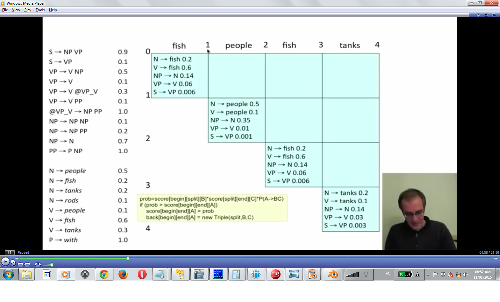
- first apply all unary rules to the words; cells in diagonal of the parsing triangle are filled in. (keep backtraces to get the result (like with edit distances)
- then fill the inner nodes: reduce input from bottom up and from left to right( node(1,0) node(2,0) ,
- for inner nodes upward: try to combine existing parse trees of given length; for word1...word3 -> try tree(word1) tree(word2..3) and tree(word1..2) with tree(word3)r
for node(2,2) then this one can be parsed by combining node(0,0) and node(2,1) (cor by combining node(1,0) and node(2,2) - difference in choosing the 'split point' along the x axis)
if two productions from the same left hand side are possible: chooses the result with highest probability:
(15-5 evaluating parsers)
- Label precision: compare with parses in treebank; each node (constituency) and its positions are recorded (NP (2,4) VP (5,7); compare number of coinciding nodes between tree bank parse and parser
output. as usual computer precision/recall.
- for wrong noun phrase attachment the result will be low (cascading errors through the nested tree)
- P (probabilistic) CFG: result will be 73% for F1 measure; not great; at least it tries to deal somehow with grammar ambiguity.
- very bad as language model: because of being context free (likelihood of rewrite rules is not conditioned on words that make up the production); (even n-grams give better results)
(16-1 lexicalized PCFG's)
- lexicalized CFG: for each category name (VP,NP) add the head word of the current clause as it appear in parse tree to category name;
Define head word for NP: (NP-)
head of VP : (VP-)
S : (S-)
PP : (PP-)
Problem: number of non terminal explodes ! Advantage: can condition probabilities of a parse on its head words: can condition PP attachment for particular prepositions/head word combinations. (does
PP attach to VP or NP?)
(16 - 2 Charniak model for PCFG's (1997))
- parsing from bottom up (like CKY)
- probabilities condition from top to bottom (need to know probability of parent node prior to finding probability for node)
- P (h | ph , c, pc) : probability of head word h word of a parse node is h : condition given the probabilities of ph - parent head node's head word; c - category of the node ; pc - parent category
of the node)
- P (r | h, c, pc) : probability of production rule : conditioned on given probabilities of head word (h); category ©; parent category (pc)
(S (NP VP))
S - has pc (parent cateogy pc - S) ; ph (parent headword)
NP - - has h - headword; c - category (NP); r - production rule chosen to expand NP
- the aim: to know the probability of expanding a given word with a given rules.
(? does that scale to large corpus ?)
- problem: hard to predict likelihood for probability distributions: things get very sparse;
- solution: (like with language models) interpolation between different models
P (h|ph,c,pc) = Lambda-1(e) P-MLE(h|ph,cpc) +
Lambda-2(e) P-MLE(h,C (ph),c,pc) +
Lambda-3(e) P-MLE(h|c,pc) +
Lambda-4(e) P-MLE(h|c)
(what a mess, probably only good for small corpus/tree bank)
(16 - 3 independence assumption of PCFG's)
- independence assumption in pure PCFG's - no assumption on context; only looks at label of the node; content of node is of no interest to the model.
- that's to tall: NP under S or NP under VP: likelihood of productions for each of these cases is very different.
- als PCFG's do not perform too well (often choose the wrong parse as the most likely one)
- really need context to disambiguate posessive NP ; ( ( NP (NP (Fidelity) POS ('s)) II (new) NN (toy))
((NP (NNP Big) (NNP Board)) (JJ composite) (NN trading)) <-> (NN (NNP Big) (NNP Board) (JJ composite) (NN trading))
- what helps is state splitting (Johnson 98) to non terminal name - add name of parent non terminal ((S-ROOT) (NN-S) (VP-S))
- problem: too much state splitting leads to sparseness of probabilities (bad) need smoothing, etc
(16 - 4 Unlexicalized PCFG's)
\[Klein Manning 1993\]
- does not add head word to non terminal
- allow more states (like NP-S but do not add all of them wholesale); or add other features NN-CC (CC - coordinative noun phrase)
- target: make limited number of state splits (to keep grammar small and fast (and prevent smoothing))
- assumption: most of the state splitting consider/take into account grammatical features: finiteness, presence of verb auxiliary.
- other work: (Charniak Collins):
Problem: rules like NP = NNP NNP NNP; these rules are split to binarization; this creates deep nesting structures so
that probabilities get split so that they get very small (they are multiplying probabilities in PCFG);
Solution: only consider 1 or two adjacent expansion (Markovization - consider only limited context;see 'memory assumption of markov models')
Horizontal markovization: for long rules consider only probability first of first two non terminals
Vertical markovization: also look at probability of parent category (or also parent of parent))
- other problems: unary rules (like S : VP ) are used to swap categories, so that a high probability rule can then be used on the sub tree for the right hand side of the unary rule)
problem that these unary rules do not apply for specific context
solution: add context that say when to apply unary rule (by state splitting S, S-U where to allow uniary rewrite)
- other problems: tree bank cateogories (non terminals) are to coarse (example: tree bank IN is used for sentence complementizer (that weather, if) ; subordinating conjunctions (while after) and
true prepositions; fix is to subdivide the IN category.
- PP attachment problem: want to know if PP attaches low or high in the phrase; so that can be conditioned on the verb that appears with the NP
(16 - 5 latent variable PCFG)
- \[Petrov and Klein 2006\] tries to do state splitting by machine learning (unlexicalized categories)
- for each category: tries to split categories if performance is improved, keep it else roll back. (does not go into the details)
- resulting splits reflect semantic categories: (proper nouns, first names, second names, place names) same for pronouns
(17 - 1 Dependency parsing)
- Head word/governor is the node;
- node points to its dependents
Result is a tree (that means no cycles and one head)
by convention they have a ROOT node that points to head of the sentence
= how does that relate to context free grammars? Nowadays categories are annotated with the head word (lexicalized CFG's; x-bar theory); so one assumes that there is dependency between nested
consistencies then CFG is a kind of dependency grammar.
- difference: dependency grammars have more flat parse tree:
CFG: (S-walked (NP-sue) (VP-walked (VBD-walked) (PP-into ))) ;
in dependency grammar walked is dependent directly on on sue; walked; into.
- in dependency grammar you can point across spans (crossing dependencies); however CFG is strictly subtree, can't do that.
- dependency parsing: one possibility is dynamic programming with CKY; or maximum spanning tree algorithm
- preferred: left to right parsing (! MaltParser does O (1) !)
- what are the features available ?:
Valency of heads: how many dependency are usual for a head? are Dependencies attached to the right or left of the word?
dependency distance (mostly within nearby words ?) (? true for languages with free word order ?)
bilexical affinities: pair or words that usually appear together (the <-> issues)
intervening material: dependencies rarely cross verbs or punctuations (commas they do cross)
(17 - 2 Greedy transition based parser (example: MaltParser))
- makes local (greedy decision)
- left to right 'shift' 'reduce' parser; has a stack
- Shift: take next word in input and push to stack
- Reduce: take next input word and a term on the stack (DG: the dependents/CFG: the left hand side of a production) and combine them/reduce it to one symbol; put result on the stack
(DG: the head word/CFG: the right hand side of production)
Left arc reduce: (adds <- arrow) take word to the right as head
Right arc reduce: (adds -> arrow) take word to the left as head
(also need to attach label on to the resulting arc)
Problem with this approach: if all the arcs point to the right then have to shift all words until the last one, then reduce reduce reduce; (Lots of shift means large lookahead: hard to tackle with
machine learning techniques).
- Solution: arc-eager parsing:
Idea: allow to establish right arch dependencies before they are fully resolved
- Left arc reduce (builds <~~) again between \[input word\]<~~\[head of stack\] ; only if \[head of stack\] is not already head of dependency (rule to prevent situation that stack is pointed to by two
arrows)
- Right arch reduce (builds ~~) reduce \[input word\]~~> \[head of stack\] ; also take \[input word\] and \[push it to stack\] - so that it will find the head word of this clause !
- extra reduce: once the head word has been found; reduce this word of the stack.
- to decide if to reduce and direction of arch: train classifier with maxent model that decides on the local step. Available features: top of stacks, POS, first in buffer, its POS; length of arc,
words between arcs. etc.
- O (1) - only greedy/local decisions made at each step ! and that's almost as good as the best LPCFG and its much faster.
Evaluation of parser performance: each word in sentence is numbered : 0 - Root of sentence; 1 - first word; for each word: what is the index of its head? what is the function of the word?
as usual: Accuracy = \#correct dependencies / \# of dependencies;
Problem in dependency parser: crossing dependencies
who did bill buy the coffee from yesterday
buy: head of ,did ,bill, coffee, from, yesterday.
but who is the heda word of from ! this is crossing dependency that spans across the tree (can't have that with CFG)
Now arc eager parsing can't do that (area of research)
(17 - 3)
one of the advantages of dependency trees is that they map naturally into a semantic representation (CFG would require additional 'deep structure' transformations over the parse tree, just to make
sense of the structure !)
- example: task of extracting interactions between genes/proteins from biomedical literature:
picture dep-1
the verb interacts indicate relations; dependencies indicate subjects and objects of interactions. (see conjunction that indicates two objects)
- stanford dependency representations: represents dependencies as projective dependency tree (can get it from post processing of penn tree-bank)
(jumped (boy-nsubj (the-det) (little-amod)) (over-pre (the-pobj (fence-det))))
boy-nsubj : nsubj - the label of the arch between jumped and boy
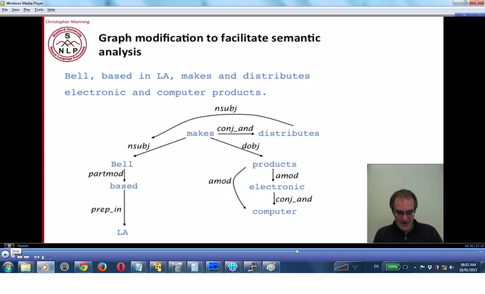
- other changes made for relation extraction:
- collapsing nodes (based (in (LA)) -> (based (LA-prepIn))
conjunction: both makes and distributes point to subject (now it's a graph and not a tree)
- looking at results of BioNLP (competiton of relation extraction in bio):
- Most relations are 1-3 dependencies away; but linear distance between the subject and object is up to 5-6 words;
- this means that dependency representation is very efficient (shallow tree is easy to inspect for semantics step)
(18 - 1 information retrieval)
- works on large collection of (usually) unstructured text (set of documents)
- task is to satisfy a information need and to find relevant information from this heap.
Workflow: user has a task; formulates an information need; then formulates a search query; query is passed to search engine, based on results the user may have to revise previous staps
Evaluating search results:
Precision := number of relevant documents returned by query / number of results returned by query
Recall := number of relevant documents returned by query / number of existing relevant documents
(Problem - these are subjective with respect to users information need, these are low if query is not well formulated)
(18 - 2 term document matrix)
- rows of matrix: all words in the corpus (lower case, after stemming to keep count low)
- columns: all available documents
- matrix\[i,j\] = 1 if word i occurs in document j
- very sparse, so it is impractical to store such a structure
(18 - 3 inverted index)
- each document identified by document-id (serial number)
- for each term in corpus (lower case after stemming): keep list of document-id's where term occurs in. (sorted by document id)
- term1 and term2 := because list is sorted by document-id: merge list and return documents that occur in both lists
which terms are indexed (have a list of document-id's where they occur?)
- text is tokenized (John's -> John, state-of-the-art (remove hyphens); remove punctuations.
- normalization: U.S.A -> USA; stemming
- olden times: remove stop words (the, a, to, of) ; now they don't do that because it kills phrase searches
Processing:
after that sort terms of each document: then produce pairs (term, document-id); then sort-merge all pairs of (term,document-id) (stable sort so that documents are lined up by document id)
- they try to compress the indixes, because they take up a lot of space.
(18 - 4 query operations)
- term1 and term2 := because list is sorted by document-id: merge list and return documents that occur in both lists
(18 - 5 phrase queries)
- possible solution: add bi-word index (each bi-gram as entry in index); then each for (query-word1 and queryword-2) and merge with (query-word-2 and query\_word-3)
- problem: not quite exact: can have false positives for words do not appear in adjacent positions.
- problem: index much more massive (not good for tri-grams)
- Positional index: need to extend inverted index: in addition to document id need the position of match in document pair : document-id:position-in-document
- these also need to be sorted by position (doc-id-1:1, doc-id-1:10, doc-id-200:5, doc-id-200:55, doc-id-200:402 )
- for matching document: merge the position list in the same way to find adjacent matches.
- can also do proximity queries: term1 within n words of term 2
- problem: positional index is larger (especially with long documents) than simple inverted index. Positional index 2-4 times larger; and is now about 35-50% of original text size !!!
- combined approach: add common bi-gram's (appear frequently as search terms) to index ; claims it uses 26% more space but 1-4 of the time to process)
(19-1 ranked retrieval)
- boolean search: difficult for users to handle; return too many (typical for or query) or to few results (typical for and queries)
- need more relevant results to appear on top/at the beginning of search result list
- assign score to documents: 0..1
- (altavista) for single word queries: 0 - word does not appear in document; >0 word appears in document; higher result if word appears more frequently (or in the beginning or in the
title)
(19-2 Jacquard coefficient)
jacard(A,B) = | A n B | / | A u B | (number of elements in intersection divided by number of elements in union)
0 - for disjoint sets ; 1 if A eq B ;
Problems:
- does not consider term frequency;
- also search terms with rare frequency (\# of occurrences of term) are more informative then terms with large frequency (jacquard does not take this)
slightly better measure:
jacard(A,B) = | A n B | / SQRT( | A u B | ) \# size of document should not skew results by much
(19 - 3 Term frequency weighting (TFW))
- assume we know how many times a term occurs in document
(do not consider order of words - bag of words model - this has its limitations, as positional info is not considered)
- assumption: documents where search term occurs a lot is preferred over documents where search term occurs just once (however measure should not grow linearly with occurrence count)
- treat words in document as bag of words (order does not matter) (? this throws away useful information: does not assign higher weight for words that appear in title or first passage?)
also term frequency Tfd
count-of-term-in-document
- take 1 + log( count-of-term-in-docubment ) \# if count-of-term-in-document > 0 (log - base 10.)
0 \# count-of-term-in-document == 0 (because log(0) = -infinity
sum that over all search terms in the query.
document sore of document that matches search query
(sum-over-term-in-query-t ( 1 + log-10 ( count-of-term-in-document-that-matches-sarch )
(19 - 4 term frequency/document frequency weighting (TF-IDF weighting)
- assumption: rare words more informative than frequent words; give high score for rare words
document=frequency( term )
number of documents where term occurs in \# the more this count, the less the information value of a term
- want inverse of document frequency (IDF): the less the count the higher the score
inverse-document-frequency( term )
log-10 ( Number-of-documents / document-frequency(term) ) \# log to dampen the effect
- score( query-result) = sum-over-search-terms-that-appear-in-query-results( inverse-document-frequency( term ) )
\# so that the score is only affected if there is a multi-word query (so it is useless with AND queries?)
(19 - 5 TF-IDF weighting)
TFxIDF (term, document) = term-frequency( term, document ) \* Inverse-document-frequency( term ) =
(1 + log( count-of-term-in-document ) \* log-base-10( Number of documents / Number of documents where term occurs in (DF (t))
- this is the best measure so far (most commonly used)
- the value increases both with frequency of term and with the rarity of word in a document.
score of a query
the sum of TFxIDFscores for each of query terms.
(19 - 6 cosine scores)
Vector space := dimension: (t1,....tn) where n is number of terms in corpus/index;
each document is a point in this space (x1...xn) where xi - number of occurrences of word ti in given document.
Queries: also vectors (t1. tn) ti - search term in query; each search match also represented in the same way.(that's more practical)
distance between two vectors in in this vector space?
- euclidian distance: (not good if some search terms have high hit count); so vector has to be normalized:
- use angle between normalized vectors (vectors of the same length) (all xi divided by length of vector)
- so they use the cosine of the angle (cosine property: monotonically decreasing for 0 ... 180 degrees; only angles between 0 .. 90 - as all counts are positives.)
- for vectors x, y : cosine(x,y) = (X \* y) / ( |x| |y| ) \# linear alg: x \* y - dot product ; |x| - euclidian length of x.
- for search term (t1...tn) take vector q=(x1...xn) where x1=1...xn=1;
- for each search hit measure cosine between normalized vector for search hit and q vector; (smaller angle means higher value)
(19 - 7 use tf-idf and cosine scores together)
- there are many variants of term frequency weighting (taking logarithm of inverse term count is only one way of many);
- the SMART information retrieval system had a lot of influence here.
- how they compute the score (again):
- represent query as term frequency vector t1, ... tn - search terms of queries so this - its value is identity vector (each search term occurs once)
- compute inverse document frequency vector for each search term
- compute cosine between each search result and the identity vector (identity vector - which we have called the term frequency vector)
- sort search results by cosine value
(? position of a word in document is not evaluated: altavista used to assign higher ranking to documents with query terms in title; also no word of page-rank ?)
(19 - 8 evaluating search engines)
- want to measure user happiness / relevance of search results to users information needs (hard to quantify)
- so they assemble following test data:
- benchmark document collection and benchmark query collection
- by hand assign which documents are most relevant to a specific query
- run the system through this test set and measure precision/recall/F measure
- another measure: mean average precision (wants to consider quality of the first k top results)
- for each query in the benchmark set
- for each set of the first n query results (up to the limit k)
- compute precision of this set (\# relevant results / size of set)
- compute average over the computed precisions (this is called mean average precision)
- then average over all mean average precision results for all benchmark search queries.
(20 - 1 Word senses and word relations)
Some definitions:
lemma/citation form := same stem, part of speech
wordform := an inflected form as it appears in text
word sense := description of one interpretation/apsect of the meaning of a word
(word : description)
Homonym := a word that holds multiple meaning;
Homophones := two words sound similar but have different meaning (Piece and peace)
Homograph := same word but holds different meaning (bat - club, bat - animal)
Polysemous word := word has multiple related meanings (bank - building of a bank; bank - financial institution)
Systemic polysemy := same pattern of different meanings (School,university,bank - can mean both building and institution) (this is also called systemic relationship
Test that word has more then one sense/meaning - zeugma test: construct a sentence that uses two meanings of the same word (construct the sentence out of two sentences with the same word)
"Does Lufthansa server breakfast and San Jose" - sounds weird, so there are two senses.
programs that process text have difficulty with ambiguity introduced by Homonyms.
two different words can share the same meaning (same meaning when the words are used in some specific contexts.
two lexemes have the same propositional meaning (are synonyms) if one can be substituted for the other in all situations (this is quite rare, so these are perfect synonyms vs. imperfect
synonyms that do not match in all situations (not acceptable in all situations)
(big,large synonymous when speaking about things (sense: older, grown up); large-sister - different meaning from big-sister (does not have meaning of older, grown-up)
Antonyms - two words with the opposite meaning (with respect to some particular meaning)
- can be at opposite ends of a scale (fast,slow)
- define a binary opposition (black white)
- can be reversed (or different directions) rise/fall up/down
hyponym := sense-a hyponym of sense-b -> if sense-a is in subclass of sense-b (car hyponym of vehicle)
(also denotes IS-A relationship between sets: A IS-A B (if x is in (is a) A it follows that x is in (is a) B) (another term: B subsumes A)
hypernym/superordinate := the reverse (vehicle is hypernym of car)
(20 - 1 Thesauri)
Thesauri/ontologies - repository for meaning (a categorisation that has the words as leaf nodes ? the categories are supposed to denote the meaning)
Wordnet:= thesaurus with aspect of dictionary. For each word there is a definition and its ontological relationship (part of speech; and IS-A/is instance of)
in wordnet a sense of a word is defined as a synonym set (set of words with the same description(gloss); these words would act as synonyms when used in a specific context, this context is defined y
the shared description/gloss)
Thesaurus := hierarchically organized lexical database (groups togather words by meaning)
Other relationships in wordnet :=
Hypernym, Hyponym, Member Meronym (Has-Member); Has-Instance; Instance-of; Member Holonym (Member-Of); Part Meronym (Has-Part) Part Holonym (Part-of); Antonym
Mesh := medical subject headings thesaurus
(he does not mention Roget's thesaurus)
(20 - 3 use a thesaurus to compute if words are similar)
word similarity := near synonyms
related words := linked by some chain of relationships as taken from thesaurus.
algorithms for computing similarity
- thesaurus based: look at the chain of links (length of the chain) between two words; do words have similar glosses/descriptions?
- distributional algorithms: look at statistical distribution of two words, are they similar?
thesaurus based/Passed based similarity - look at the length of the chain of relations that is linking two words
pathlen(s11, s2) = 1 + number of edges in shortest path in hypernym graph; where s1,s2 are two word senses/glosses.
simpath(s1, s2) = 1 / pathlen(s1, s2) \# want to make a value between 0 .. 1 (there is always some length != 0 because all senses are linked via the root category)
wordsim(w,w2) = maximum( foreach-word-sense-s1-ofw1( for-each-wordsense-s2-of-w2( simpath( s1, s2 ) ) )
Problem: each links are assigned the same distance; however links closer to the origin concept should have higher weight as they are more relevant, less abstract.
words( concept ) := look at subtree of words and concepts in thesaursus; take number of words and concepts in this subtree
Probability that a word belongs to a concept.
P( concept ) := words( concept ) / Number-of-words-in-corpus (? shouldn't that be sum of words and concept of a thesaurus ?)
Information-content( concept ) = - log ( P( concept ) ) \# just like in information theory
Lowest-common-subsumer( concept1, concept2 ) := lowest parent in thesaursus that is above both concept1 and concept2
Resik mmeasure: if two concept are linked via closer ancestor then they are more common.
Similarity-Resnik( concep1, concep2 ) = - log( P ( Lowest-common-subsumer( concept1, concept2 ) ) )
alternative Lin similarity measure (didn't quite understand that)
alternative: Lesk similarity measure: does not look at hierarchy, only looks at the description/glosses of concep1 and concept2
- for each sequence of words that appears in both gloss of concept1 and concept2 - add length(sequence of words ) ^ 2 to measure
- in some variations also compute this measure for hypernyms and hyponyms of concept1 and concept2 and add them to the resulting measure
Evaluation: intrinsic evaluation (compare with test set rated by humans); or extrinsic evaluation (plug it into a task and see if task performs better with new measure)
(20 - 4 word similarity - distributional methods to compute word similarity)
Thesaurus is not always available, or it lacks a given word/meaning, etc.
distributional methods do magic over vector spaces (like in information retrieval), however precision is lower then with thesaurus based methods.
Rational: if a word appears in the same context (near similar words) then it is counted as a synonym (Firth:1957 - 'You shall know a word by the company it keeps')
Intuition: word document matrix: rows of matrix - set of input words : we try to compute the similarity between these input words; columns: all documents; cells: count of word (column) in
document (row)
Now instehad of documents for rows we take more limited context: one passage or 10 words within a given word (? which set of words are chosen to form these contexts ?)
Also instead of word counts they are using the 'Pointwise mutual information' (PMI) measure - this measure is high when two event occur both, and low if not (events not correlated)
PMI( word-x, context-y) = log-base-2 ( P (word-x,context-y) / (P (word-x) \* P (context-y)) )
\# if word-x and context-y are correlated(word-x appears a lot in context-y) then its probability is higher and p(word-x, context-y) is higher
\# positive PMI (PPMI) - if logarithm is lower than 0 then return 0.
P (word-x,context-y) = (word-count\[ word-x\] \[context-j\] / sum-of-all-wordcounts-in-matrix) / P (word-x) P (context-y)
P (word-x) = sum-of-word-counts-in-row-for-word-x / sum-of-all-wordcounts-in-matrix
P (context-y) = sum-of-word-counts-in-column-for-context-y / sum-of-all-wordcounts-in-matrix
\# PMI has bias towards infrequent events, so use +1 smoothing (or +n smoothing)h
- like in search engines: use arc cosine to measure distance between these normalized vectors.
(20 - 5 word similarity - distributional methods 2)
better way, two ways are similar if they appear in similar parse context: (similar prepositions; similar head words, similar dependents)
so columns of matrix look as follows: subj-of~~word> modifier-of~~ ; obj-of- etc.
- like in search engines: use arc cosine to measure distance between these normalized vectors.
(21 - 1 question answering)
question answering (1961:Simmons) ; parse question into dependency graph/tree; find matches of this dependency tree in database;
IBM Watson (2011); Siri (can ask factoid questions: Where is the Louvre? bit more complex one "do i need an umbrella tomorrow?); Wolfram Alpha")
two approaches:
- Information retrieval approach :
process question:
- try to detect answer type; domain of question (which one of the available data sources can answer the question)
- build information retrieval query
passage retrieval (information retrieval step)
- fetch query result and break up into passages.
answer processing
- extract answers from search result (ppassages) and rank answers
- hybrid methods
build shallow parse tree (constituent noun/verb phrases but do not parse the whole thing); use that for the usual query type detection;
use question to formulate multiple queries to information retrieval system (find candidates); so they have a lot of candidates
evaluate the answers by correlating it with specialized databases (geospacial DB; thesaurus/taxonomies; use temporal reasoning)
(use knowledge based methods for scoring answers)
parse tree/dependency tree of the question; build semantic representation for it; and find answer based on that methods to score answer
the system has semantic representation of questions that it understands/is able to answer; and it matches the parse tree of the input question to one of these.
(21 - 2 Information retrieval approach: step of processing input query: answer type detection)
- answer type detection
what kind of answer is expected in the question; does it want to find out a person name or place name? etc. etc.
A taxonomy of questions is used here (Li,Roth 2002)
6 coarse classes (ABBREVIATION,ENTITY,DESCRIPTION,HUMAN,LOCATION) these are divided into 50 finer classes (example: ENTITY: animal, body,color,currency (? what kind of taxonomy is
this?))
For IBM Watson they found 2500 answer types; most frequent 200 types covered <50% of Jeopardy questions.
can be done by hand written rules with regular expressions (who {is|was|were|are} PERSON)
first word of a query is often head word of a noun phrase (which city hots the olympics? -> which ; look at dependents of head word.
machine learning: train classifiers from training data (to assign one of the question categories from a taxonomy)
- query formulation
extract query that is to be passed to information retrieval system (aka. search engine)
as usual: heuristics x
- remove all stop words (a, the)
- in quotes - good indicator that this is part of query
- NNP words in recognized named entities
- nominals with adjective modifiers
- nouns
- etc. etc.
Any selection of these combinations (from first - highest priority to last)
- question type classification
is geo spacial data requested, or is it about restaurant reviews?
(if yes use specialized database, or specialized search engine for information retrieval; etc)
- focus words
which words within the question will be replaced by fact that is returned as the answer? (for formulating an answer)
- relation extraction - between parts of the question; these relations extracted are logical constraints that are used to filter out/evaluate an answer from search results
(21 - 3 passage retrieval + answer evaluation)
processing of query results returned by search engine:
- partition into shorter sections (paragraphs)
- check if any of the passages contain an answer to the question
Features tocheck:
- \# of named entities of requested type in passage
- \# of query words
- \# of n-grams from question
- proximity of keywords
- longest sequence of words from question
- etc. etc
evaluate is a passage contains an answer to the question
- can use named entity tagger: extract words with same tag as requested answer
- problem: a passage contains multiple answers; (again train classifier etc. etc.)
In Watson they have 50 different components; each one responsible for heuristics regarding one type of questions
for remaining ambiguities they use a magic ranking system to sort it out (mean reiprocal rank - did not quite understand that one)
(21 - 4 using knowledge in question answering)
- relations that have been extracted from wikipedia born-in(x,y) author-of(x,y) ; etc.
- temporal reasoning: when did AAA live? as a hint if AAA is a good answer to a question
- geospacial db: (which country is to the north of Vietnam?)
There are systems (SIRI) that allow reference to conversational state (him, who? - was mentioned earlier in the conversation)
(21 - 5 complex question answering)
(? during the end of an NLP course they usually start to do a lot of hand-waving, isn't it ?)
(22 - 1 summarization)
summarization: given a text A; produce a text B that contains information from text A that is important to the user (B is an abridged version of A)
this can be used for the following purposes
- create outlines/abstracts of articles (reddit has this!)
- summaries of email conversations
- extract action items from meetings
- simplifying of complicated text (?is this real?)
Several kinds of summarization
- summarization of single documents
- summarization of a set of multiple related documents
other subtypes of summarization
- generic summarization
- query focused summarization: extract information relevant to a query
used in google to display a short text about the search result
(often this is extracted from a single document);
- however in order to answer complex questions we might need to combine information from multiple document (and that is multiple document summarization)
two options to do summarization:
- extractive: pull out some sentences from the original document to produce the summary (google search results)
- abstractive: produce a summary with different wording from that of the source document (very difficult, we don't handle that here)
Abstractive summarization:
- one option is to take the first sentence from a document (good baseline algorithm) (and to mark terms of query as bold)
(22 - 2 generating snippet summaries)
stages:
- content selection:
- segment text into sentences (find sentence boundaries);
- pick those sentences that are relevant
- information ordering:
- select some most relevant sentences from those picked during previous stage
- choose the order of the resulting selection
- sentence realization
- might change the result somehow (might even simplify them sentences!)
Most search engines do only content selection:
First algorithm from Luhn:1958 - choose the documents that have informative words
- can use TfxIdf (search-term, document) score (see 19 - 5 lecture)
- or use log-likelyhood ratio measure (and he does not explain what that means ! explained in Dunning(1993) )
so choose words that log-likelyhood ratio is > 10.
- adapting this algorithm for query summarization:
weight-of-sentene := ( for all words in the sentence compute the sum of the following values:
if word in query -> return 1
if log likelyhood ratio of word > 10 -> return 1
else -> return 0
) / Number-of-words-in-sentence
Alternative: supervised content selection; train one over training set
features that can be used to train such a classifier:
- position in sentence
- length of sentence
- word informativeness
Problem: hard to get good training data; Humans when they write abstract often reforumlate and choose different word sets.
(22 - 3 Evaluating summaries)
- hard to evaluate answers of sumarization (mentioned before); x
- ROGUE metric: checks what percentage of bigrams from machine generated summary appear in test benchmark summary written by a human (bla bla bla)
- this is cheaper than having a human rate the answers generated by the machine.
(22 - 4 summarizing multiple documents)
- this is an active research topic; there is a competition for that (DUC 2005 competition)
- example question: "What has caused train wrecks in recent years and what has been done to prevent them?"
two approaches:
-bottom up snippet method
treat complex question as a single question;
Search and find relevant documents; get informative sentences and order and modify these sentences
More details:
Sentence segmentation of multiple documents
Simplify these sentences
- parse sentences;
- simplify parse tree by deleting some subordinate phrases;
- what can be deleted? delete some of the modifier clauses/subordinate sentences/preposition phrases that do not refer to named entities/ adverbials (for example,etc)
- rules decide what to delete from the parse tree.
- reassemble sentence from simplified parse tree
extract relevant sentences (again by computing weights like log likelyhood, etc; and picking those with highest weight)
- for all sentences: choose sentence with maximum relevance and add it to summary
- it has to have high cosine similarity with the query
- it has to be novel (so that chosen summary has no repetitions
so it has to have lo cosine similarity with text that has been selected to act as summary at the current moment
similarity-mmr( sentence, query, current-summary ) = max( lambda \* similarity( sentence, query ) + (1 - lambda) similarity( sentence, current-summary )
(mmr stands for maximum marginal relevance)
information ordering
- harder to do with multiple documents;
- can use chronological modification date of document returned by search and order by that
- order by topic: if documents by search are classified by some keywords
Information ordering - Information extraction method
- have a taxonomy of questions; for each question type define features that make a good answer to that question
(biography answer has: birth/death, education, why is he notable; nationality, etc)
- for each question type build a classifier that can extract sentences that contain a desired aspects; then combine these sentences into an answer.
sentence realization (?not explained what that is?)
-top down information extraction
- break up the complex question into component questions (component questions may be of different types)
- query for each component question
- order so that similar sentences have similar cosine measure (); or order so that adjacent sentences have same entity mentioned (talk about the same things)